Methodology

RateProbability translates overnight-index market pricing into a simple, meeting-by-meeting view of expected future policy rate settings. The outputs are market-derived (not a forecast) and are intended to be a clean summary of what tradable instruments are pricing.

What instruments we use

Every bank on the site is priced the same way: from OIS (Overnight Indexed Swap) quotes referencing that market’s overnight benchmark (examples include SOFR/EFFR in the U.S., €STR in the euro area, and TONAR in Japan). The floating leg of these swaps accrues interest through daily compounding of the realized overnight rate over the swap period, so at any time, a quoted par rate can be assumed to reflect the market’s forward-looking view of that compounded average rate. This is the only instrument family used across every bank we cover, which keeps the underlying methodology consistent from one bank to the next and makes cross-bank comparisons more meaningful. We believe OIS to be the most suitable instrument from which to derive expectations because central banks set explicit targets for overnight rates; OIS is priced and traded by the institutions that are the overnight funding market (banks, dealers, large asset managers), with that pricing kept honest by arbitrage against repo, T-bills, and other rates products.

From OIS quotes to a curve

OIS is quoted as a par fixed rate for a given maturity. We convert these par quotes into a curve of discount factors and zero rates using standard bootstrapping logic and each market’s own conventions (day count, compounding, payment timing, and so on).

Single-payment intuition (simplified):

DF(T) = 1 / (1 + r · τ)

where r is the par/zero rate (in decimal) and τ is year-fraction to maturity.

For short tenors that behave like a single cashflow, this is a good conceptual guide on its own. For longer maturities with multiple accrual periods, we bootstrap sequentially: use earlier discount factors to solve for the next unknown one.

Rather than solving each forward segment in isolation, we build one continuous discount-factor curve from the full set of quoted OIS points and interpolate along it (log-linearly, consistent with how discount factors compound) to place any date precisely, including meeting effective dates that typically fall between two quoted maturities.

Forward rates from the curve

Once we have discount factors (DFs), we can compute an implied forward rate between two dates (t1 → t2). In a simple setting:

Forward(t1,t2) ≈ (DF(t1)/DF(t2) − 1) / τ(t1,t2)

That forward is the market-implied average overnight rate over that window (under standard no-arbitrage assumptions). This is the key object we use to connect market pricing to policy meeting windows.

Mapping to policy meetings

Policy decisions happen on discrete dates, but markets price rates continuously. We bridge the two with meeting windows: the interval from a decision’s effective date (often the next business day after the announcement—though not the case for every bank) to the next decision’s effective date, and so on down the calendar.

For each window, we use the interpolated curve to infer the market’s expected average overnight rate, then adjust for any spread between the market benchmark and the policy rate so the output reflects implied policy rates, not raw market reference rates.

Δ vs current (bps) and implied post-meeting rate

Each meeting row includes:

Implied post-meeting rate: the policy rate level immediately following that meeting, as implied by market pricing.
Δ vs current (bps): the cumulative difference from today’s reference level into that meeting, expressed in basis points. In other words: the number of basis points priced-in between now and that meeting.

“Current” means a consistent policy-rate reference for the bank (for example, an effective overnight level, a target/corridor proxy, or the bank’s primary administered rate), depending on the bank.

Converting pricing into a simplified hike/cut probability

Markets can price multiple outcomes (hold / cut / hike, sometimes with mixed magnitudes). Rather than displaying a full probability distribution, the site offers a simple translation using your selected step size (e.g., 25 bps):

Compute the cumulative change into each meeting (Δ).
Compute the incremental change from one meeting to the next (Δᵢ − Δᵢ₋₁).
Approximate “move probability” as: min(100%, |Δᵢ − Δᵢ₋₁| / step).

For example, if the market has 10bps of cumulative easing priced into the second upcoming meeting and 32bps priced into the third, the incremental move into the third meeting is 22bps. At the default 25bps step, that is presented as 88% (22 ÷ 25) probability of a cut at that meeting, and 1.28 (32 ÷ 25) cumulative cuts priced in by that point on the curve.

This is intentionally a simplification: it’s designed to be readable and consistent, not to perfectly reconstruct the full distribution priced by the market. You can change the assumed step size at any time (10/25/50/75/100bps); every probability and cumulative-move figure on the page recalculates instantly against the same underlying priced move in basis points.

From the curve to the page

The table and chart on each bank’s page present this same meeting-by-meeting output directly: implied post-meeting rate, Δ vs current, and the step-based probability and move count described above.

The Next Meeting panel translates those same figures into a picture of the two nearest bracketing outcomes (say, hold versus one hike) and how much of the distance between them is currently priced in. When the market has more than a full step priced in for that meeting, the panel simply advances to the next bracket pair (one hike versus two hikes) rather than capping out at 100%, so the bar chart and number line move continuously through that threshold.

A pricing-snapshot selector on this panel lets you re-render the same visualization against an earlier day’s curve (current, one, three, six, or ten weeks back), so you can see how pricing for a given meeting has moved over time, using the same underlying methodology, just captured at an earlier point.

Meeting liveness gauge

Trader accounts see a meeting liveness gauge on supported bank pages (currently desktop only). It condenses pricing for the next scheduled meeting into two readings: whether the meeting is live or dead, and how strongly it sits on that side.

The input

The gauge uses a single number: the probability of a move at the next meeting, calculated exactly as described in the probability section above, using your selected step size:

P = min(100%, |Δ₁| / step)

where Δ₁ is the basis points priced into the next meeting. This is the same figure shown for that meeting in the table. Hikes and cuts are treated alike: the gauge asks whether a move is in play, not which direction. The direction appears in the gauge’s tooltip.

What “live” means, and why 25%

“Live” is informal market shorthand for a meeting where a policy move is a realistic possibility. It does not mean a move is expected: a meeting can be live while a hold remains the more likely outcome. The gauge reads LIVE when P is 25% or higher, and DEAD below 25%.

There is no official or industry-standard threshold for “live,” so any cutoff is a judgment call. We chose 25% because:

It stays well short of 50%, keeping “live” distinct from “more likely than not.”
It is a simple, familiar fraction: a one-in-four chance, or a quarter of a standard move priced (6.25bps at a 25bps step).
It is consistent with published probability-language scales. By 25%, none of the scales shown below still describes an outcome as “very unlikely,” “highly unlikely,” or “almost certainly not”; each describes it simply as “unlikely” or “probably not.”

These scales were designed for climate science and intelligence analysis, not rates markets, and none of them defines “live.” We show them for context, not as the source of the cutoff.

Chart comparing how four published probability-language scales (IPCC, ICD 203, the UK PHIA yardstick, and Sherman Kent’s 1964 scale) divide the 0–100% probability range into verbal categories, alongside the liveness gauge’s six readings, with the gauge’s cutoffs marked at 10, 20, 25, 40 and 70 percent. — How published probability-language scales divide 0–100%, alongside the gauge’s six readings. Hatched areas are ranges a scale deliberately leaves unnamed. Sources: IPCC AR5 guidance note on consistent treatment of uncertainties (2010); US Intelligence Community Directive 203 (2015); UK Professional Head of Intelligence Assessment (PHIA) probability yardstick; Sherman Kent, “Words of Estimative Probability” (1964). IPCC ranges are nested and are shown by their narrowest term.

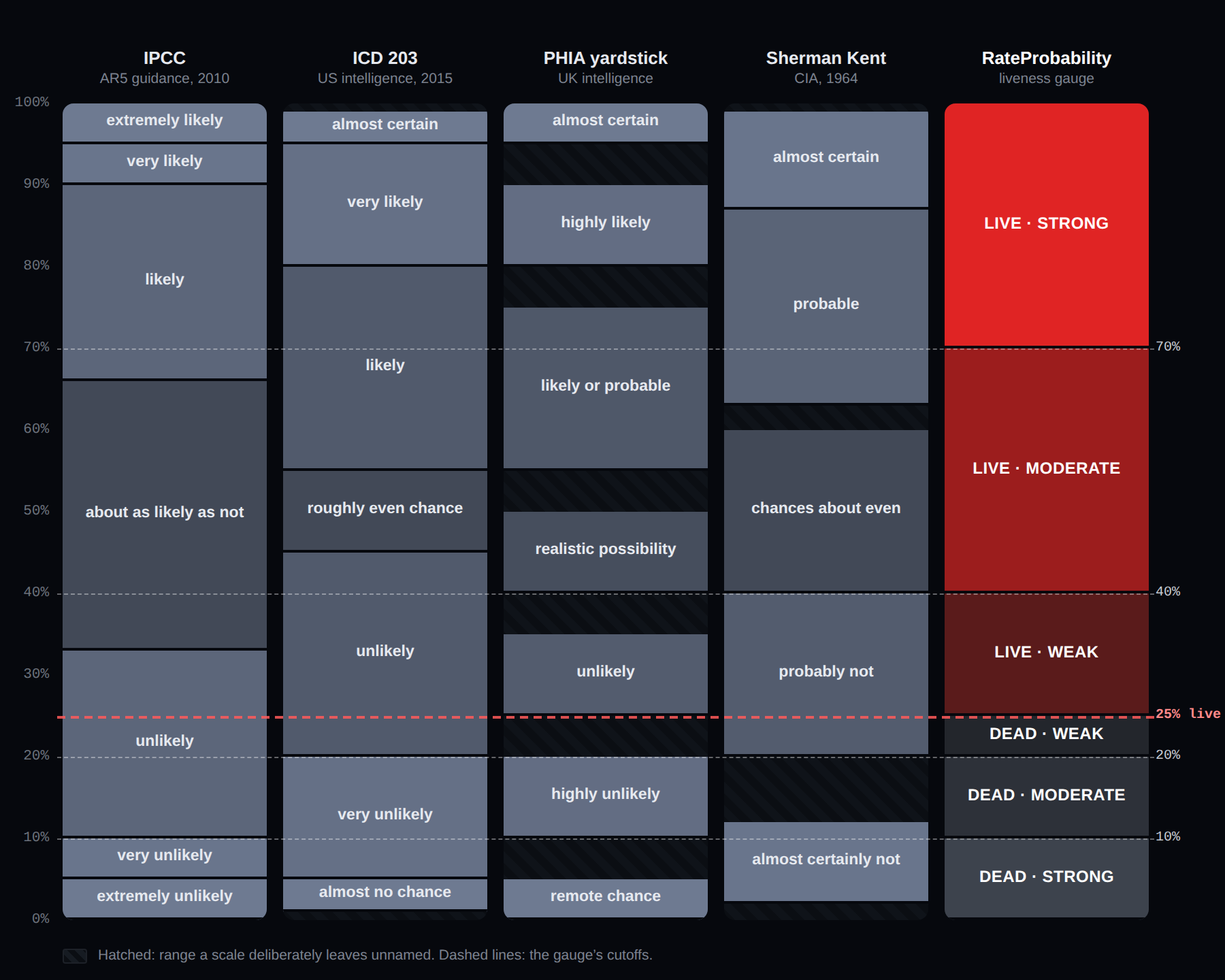
Strength

STRENGTH describes how firmly the meeting sits on its side of the 25% line. A single rule sets every cutoff: measured outward from 25%, the first fifth of the distance to 0% (or to 100%) is WEAK, the next two fifths MODERATE, and the final two fifths STRONG. Because the dead side spans 25 points and the live side 75, this gives:

DEAD · STRONG: below 10%
DEAD · MODERATE: 10% to below 20%
DEAD · WEAK: 20% to below 25%
LIVE · WEAK: 25% to below 40%
LIVE · MODERATE: 40% to below 70%
LIVE · STRONG: 70% and above

When more than a full step is priced for the next meeting, P is capped at 100% and the gauge reads LIVE · STRONG. Like the live threshold, these bands are presentation choices designed to be easy to read, not statistically derived cutoffs. A meeting crossing 25% always moves between DEAD · WEAK and LIVE · WEAK.

Strength versus Conviction

The Conviction score in the gauge’s tooltip is a separate, outcome-neutral measure, identical to the Market Conviction Index on the comparison page:

Conviction = |P − 50| × 2

It is 0 at a 50/50 split and 100 when pricing is at 0% or 100%. The two measures can appear to disagree. A meeting priced at 30% reads LIVE · WEAK (a move is in play, barely) with Conviction 40 (the market moderately expects a hold). Both are correct; they answer different questions.

Limitations

Step size: the threshold scales with your step. At a 10bps step, 25% is 2.5bps priced; at 50bps, it is 12.5bps. Use a step that matches how the bank typically moves.
Not a signal: like everything on the site, the gauge describes pricing. It is not a forecast or a recommendation.

Updates, caching, and fallbacks

Update frequency depends on your tier. Free accounts see data refreshed three times per day; Trader accounts see it refreshed every five minutes 24/7. In both cases, if a live fetch fails, the page displays the last-known-good cached copy rather than an error. Pages may also show an “edge cache” label when served from CDN caching.

Coverage across central banks

The same methodology is applied across all central banks on the site. The Fed, ECB, BoJ, BoE, BoC, and RBA are available on the free tier; the RBNZ, SNB, Riksbank, and RBI are currently available to Trader subscribers. The exact conversion from market pricing to policy-rate terms differs slightly bank to bank due to differences in available OIS tenors/conventions, but the output, an implied policy-rate path and simplified move probabilities, is meant to be read the same way everywhere.

Limitations and important notes

Not a forecast: this is market pricing, and markets can be wrong.
Meeting timing: instruments price continuous windows; meeting mapping is an approximation.
Conventions matter: day count, business-day calendars, and compounding rules vary by market.
Intra-meeting moves: policy changes can occur outside scheduled meetings in exceptional circumstances.
Step-size simplification: the “probability” is a readable summary, not a full distribution.
Liquidity conditions: during periods of thin liquidity, wide bid/ask spreads or erratic quote prints can show up as noise in the priced path, since the output is only as good as the quotes feeding it.

Intended use and disclaimer

This site is for informational and educational purposes only and does not constitute investment advice, a recommendation, or a trading signal. Always verify critical information with primary sources and your own judgment.